Self-Driving Car Engineer Nanodegree

Project: Vehicle Detection

The goals / steps of this project are the following:

• Perform a Histogram of Oriented Gradients (HOG) feature extraction on a labeled training set of images and train a classifier Linear SVM classifier
• Optionally, you can also apply a color transform and append binned color features, as well as histograms of color, to your HOG feature vector.
• Note: for those first two steps don’t forget to normalize your features and randomize a selection for training and testing.
• Implement a sliding-window technique and use your trained classifier to search for vehicles in images.
• Run your pipeline on a video stream (start with the test_video.mp4 and later implement on full project_video.mp4) and create a heat map of recurring detections frame by frame to reject outliers and follow detected vehicles.
• Estimate a bounding box for vehicles detected.

Histogram of Oriented Gradients (HOG)

1. Explain how (and identify where in your code) you extracted HOG features from the training images.

The code for this step is contained in the code cells #3 (get_hog_features) and #4 (extract_features) of the IPython notebook. Both the functions were provided and explained in the lessons and I did not need to make any changes.

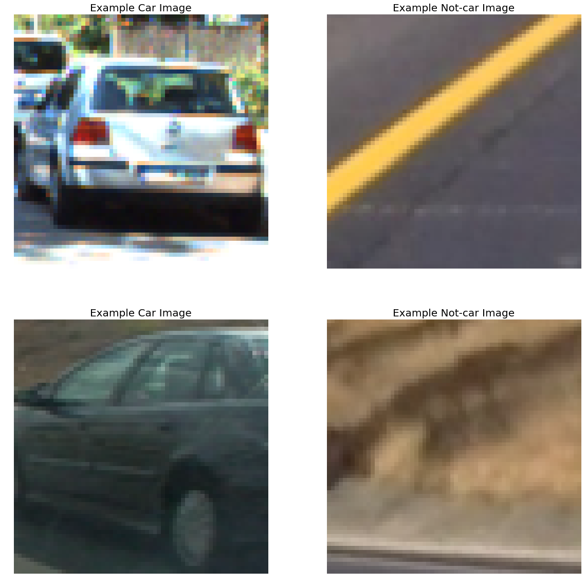
I started by reading in all the vehicle and non-vehicle images. Here is an example of one of each of the vehicle and non-vehicle classes:

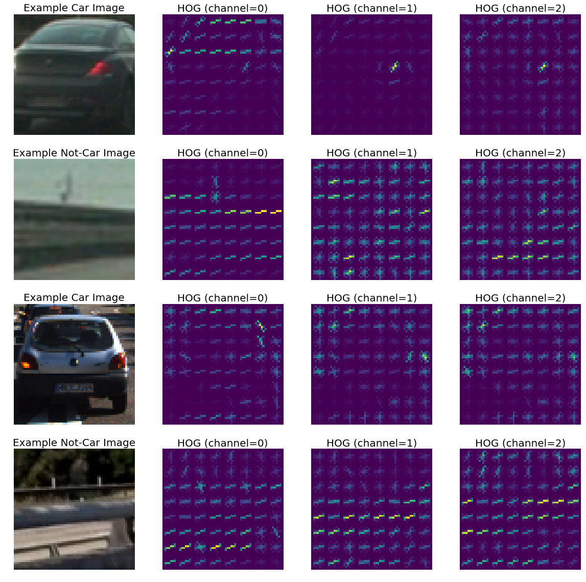
I then explored different color spaces and different skimage.hog() parameters (orientations, pixels_per_cell, and cells_per_block). I grabbed random images from each of the two classes and displayed them to get a feel for what the skimage.hog() output looks like.

Here is an example using the YCrCb color space and HOG parameters of orientations=9, pixels_per_cell=(8, 8) and cells_per_block=(2, 2):

2. Explain how you settled on your final choice of HOG parameters.

I used YCrCb colorspace and did not try others. I also used all HOG channels. I tried various values of parameters orient, pix_per_cell and cell_per_block in the classifier and settled for these parameters because they gave the best results.

### Tweak these parameters and see how the results change.
color_space = 'YCrCb' # Can be RGB, HSV, LUV, HLS, YUV, YCrCb
orient = 9  # HOG orientations
pix_per_cell = 8 # HOG pixels per cell
cell_per_block = 2 # HOG cells per block
hog_channel = 'ALL' # Can be 0, 1, 2, or "ALL"

3. Describe how (and identify where in your code) you trained a classifier using your selected HOG features (and color features if you used them).

Again I used the extract_features method from the lessons as is in code cell #4. Since the image dataset was small, I decided to use all the three types of features (HOG, histogram and spatial). I also decided to use the YCrCb colorspace because it was giving the best results. For spatial and histogram features I used the default parammeters because they were already tweaked in the lessons. For HOG I chose ALL hog channels with 9 orientations. This is because selecting a single hog channel was not working for the classifier. I used a Linear SVM which is known to work well for HOG features. I scaled the features to zero mean and unit variance using StandardScaler and split 20% of data randomly into a test set. The code for the classifier is in cell #8 of the IPython notebook.

The statistics of the whole process are printed below:

49.05 seconds to extract car features...
50.92 seconds to extract non-car features...
6.36 seconds to scale/transform features...
Using: 9 orientations 8 pixels per cell and 2 cells per block
Feature vector length: 8460
31.16 seconds to train Linear SVM...
Test Accuracy of SVC =  0.9904

Sliding Window Search

1. Describe how (and identify where in your code) you implemented a sliding window search. How did you decide what scales to search and how much to overlap windows?

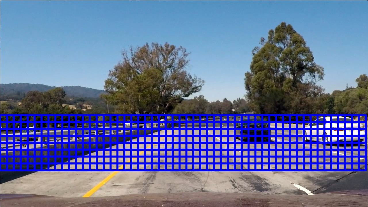
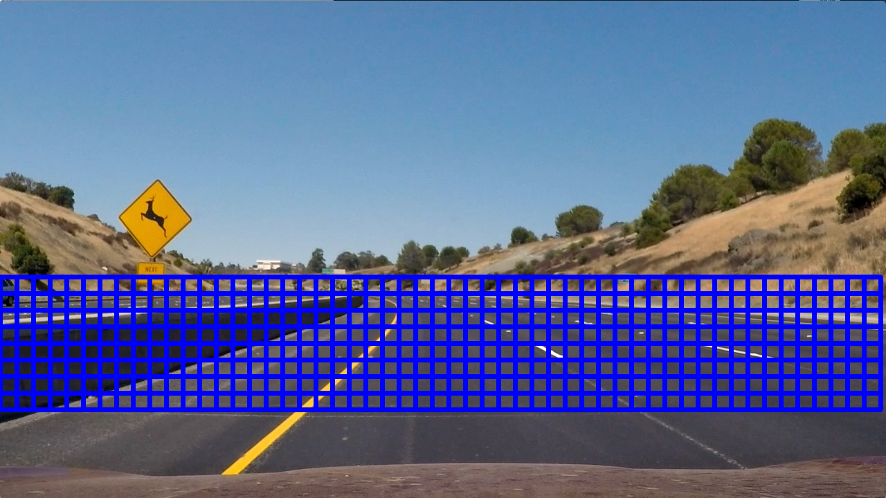
For testing on images I used the sliding_window functions provided in the lessons. Its in cell #5 of the IPython notebook. I used a single window size (96, 96), and an overlap of (0.75, 0.75). For the project I did not find the need to use multiple scales.

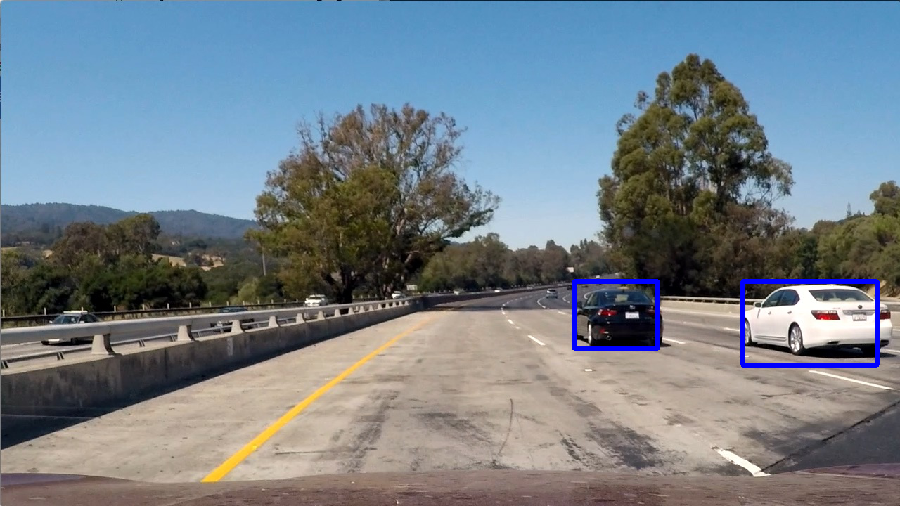
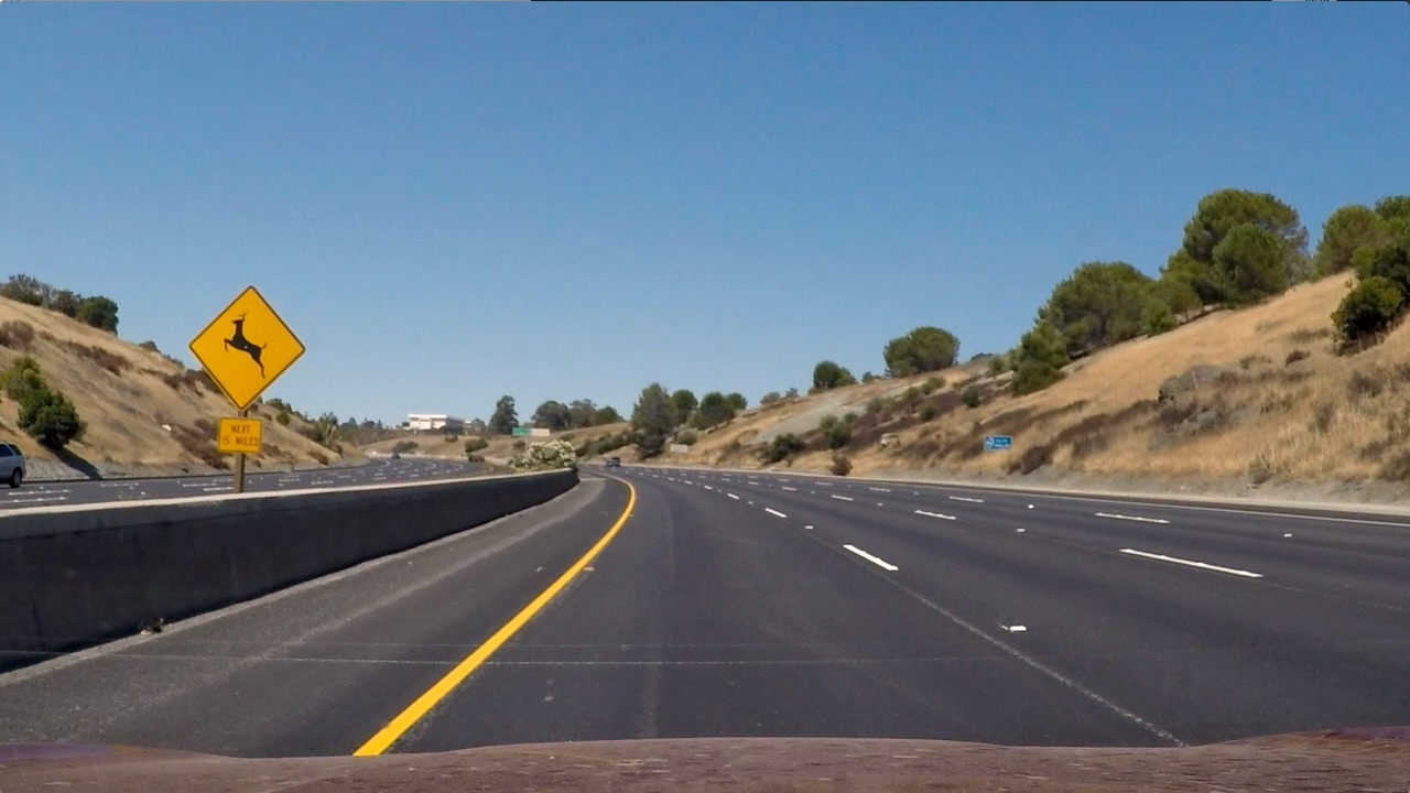
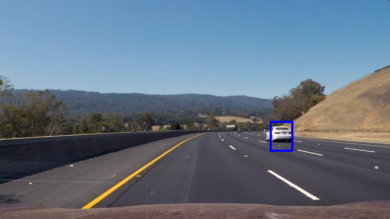
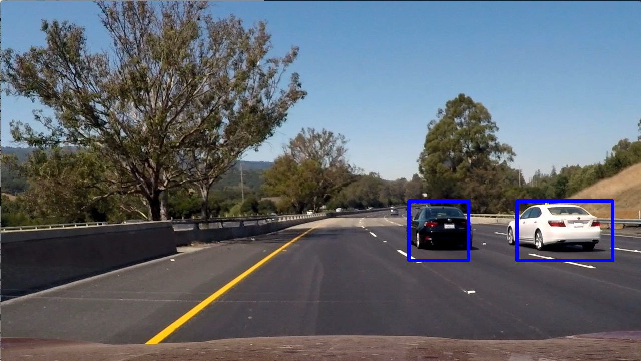
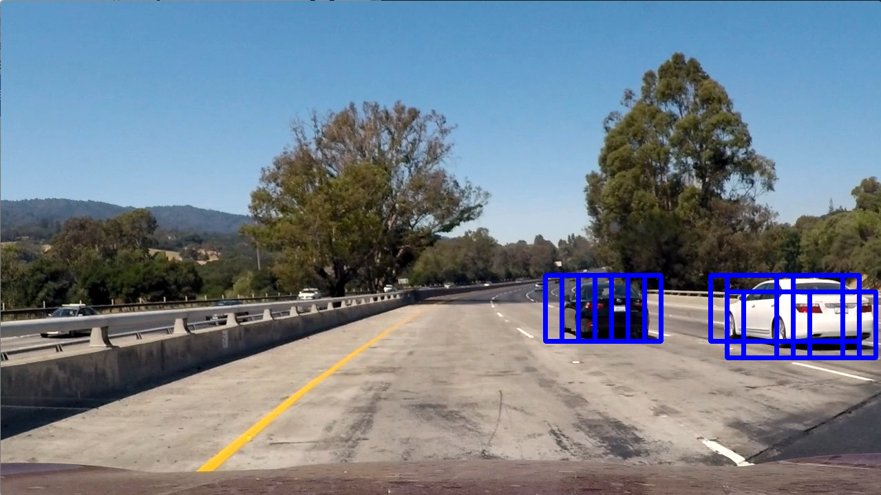
Here are the example outputs:

However for actual video processing I used the find_cars method with a scale of 1.5 (also in cell #5) because it uses HOG subsampling search and is more efficient.

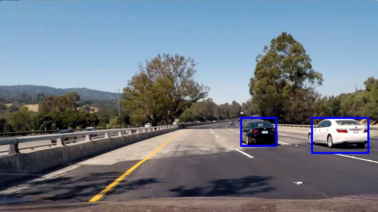
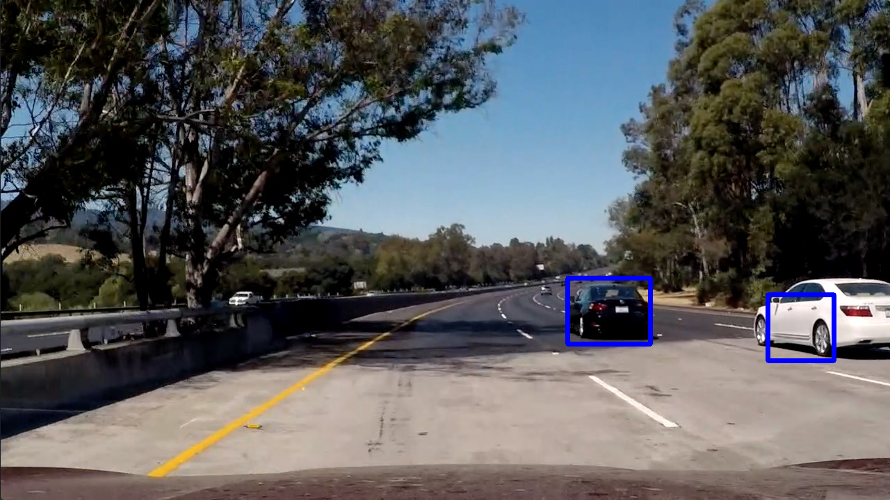
2. Show some examples of test images to demonstrate how your pipeline is working. What did you do to optimize the performance of your classifier?

I decided to use all the three types of features (HOG, histogram and spatial) so that the classifier does not overfit. I also decided to use the YCrCb colorspace because it was giving the best results. Here are the example images.

—

Video Implementation

1. Provide a link to your final video output. Your pipeline should perform reasonably well on the entire project video (somewhat wobbly or unstable bounding boxes are ok as long as you are identifying the vehicles most of the time with minimal false positives.)

Here’s a link to my video result The code for my video processing pipeline is in code cell #10 of the IPython Notebook.

2. Describe how (and identify where in your code) you implemented some kind of filter for false positives and some method for combining overlapping bounding boxes.

• I created a queue of last 30 frames.
• I recorded the positions of positive detections in each frame of the video using the find_cars method.
• From the positive detections I created a heatmap and added it to the queue.
• I then thresholded that map to identify vehicle positions. I removed detections that do not occur in atleast 15 frames as false positives.
• I then used scipy.ndimage.measurements.label() to identify individual blobs in the heatmap. I then assumed each blob corresponded to a vehicle.
• I constructed bounding boxes to cover the area of each blob detected.

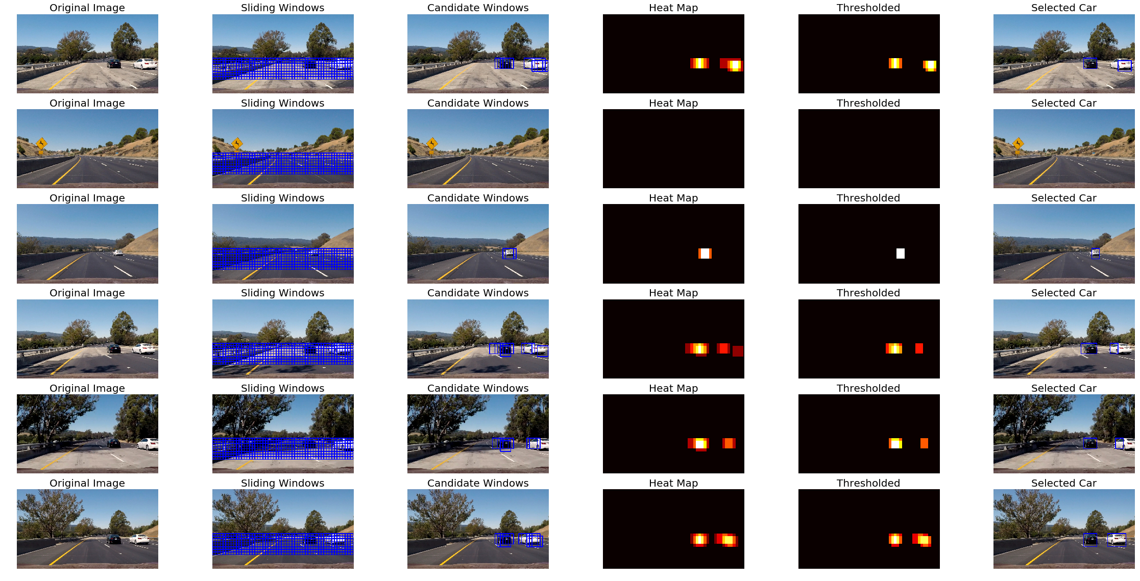
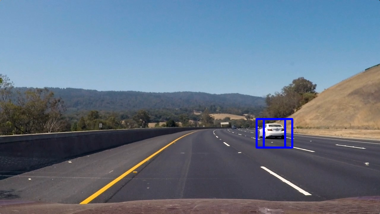
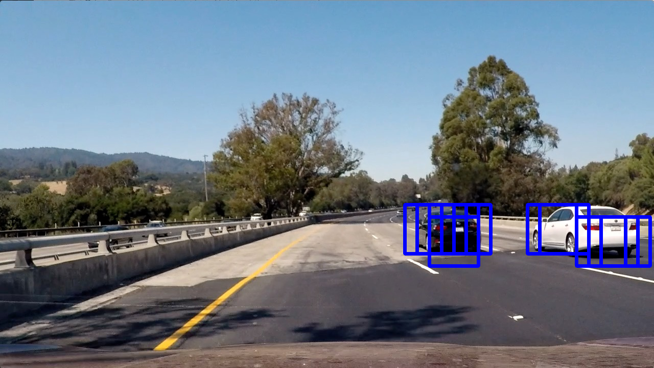
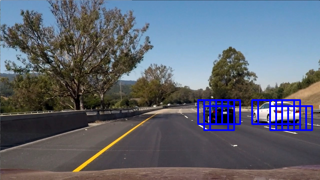
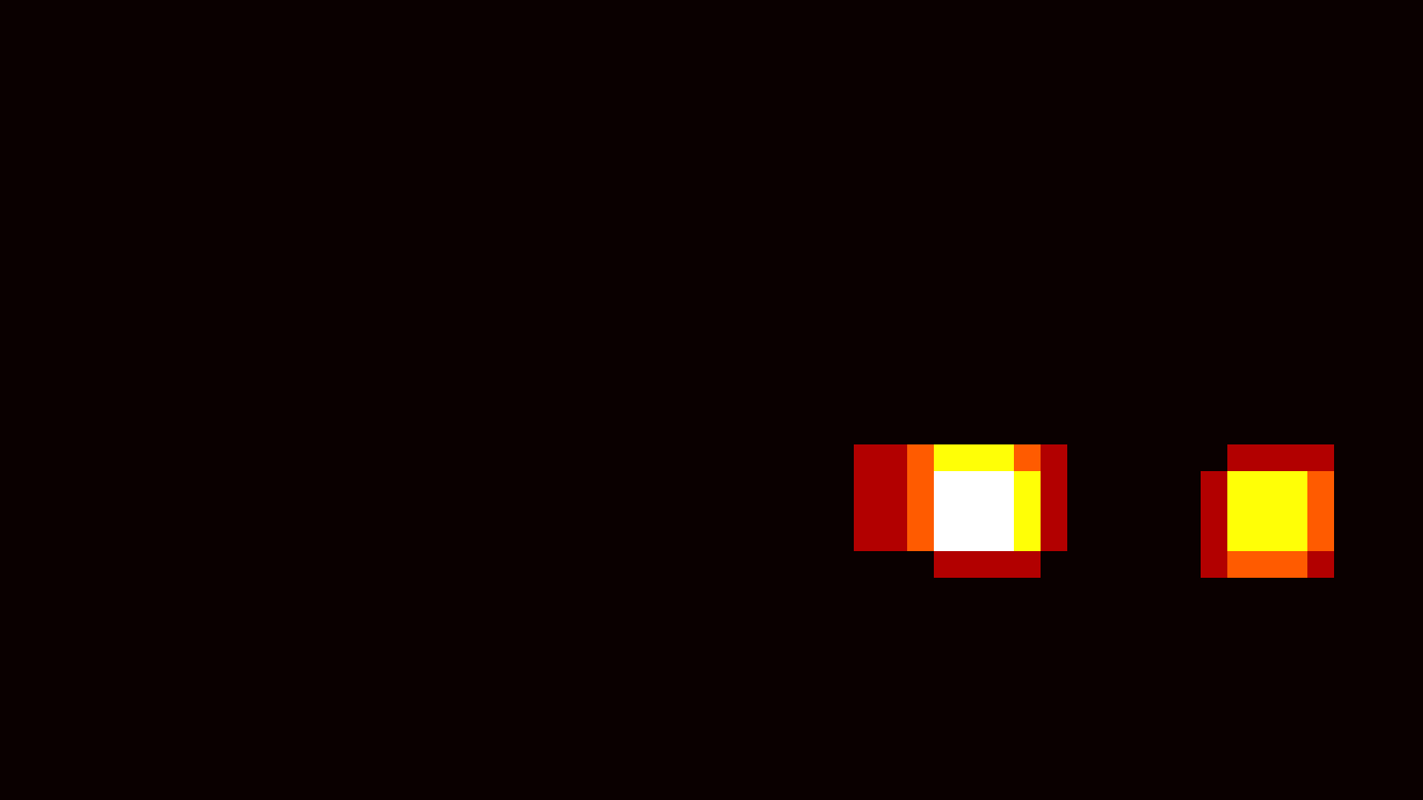
Here’s an example result showing the heatmap from a series of frames of video, the result of scipy.ndimage.measurements.label() and the bounding boxes then overlaid on the last frame of video:

Here are six frames and their corresponding heatmaps:

— —

Here is the output of scipy.ndimage.measurements.label() on the integrated heatmap from all six frames:

Here the resulting bounding boxes are drawn onto the last frame in the series:

Discussion

1. Briefly discuss any problems / issues you faced in your implementation of this project. Where will your pipeline likely fail? What could you do to make it more robust?

The great thing about this project was that most of the code was already provided and explained in the lessons. Most of the code works as it is and the only challenging part is tuning the various parameters. The only change I made is in the find_cars function where instead of drawing rectangles on the image I am returning the list of bounding boxes similar to search_windows method so that we can add heat and apply thresholds to these bounding boxes as well. The other challenge was to eliminate false positives by keeping a queue of 30 frames. Currently I eliminate any detections that does not persist for 15 frames as false positives but that may vary from video to video and can fail in cases where a vehicle suddenly comes and goes. I would like to try these things to make it more robust:

• More scales in sliding windows.
• Better handling of false positives.
• Experimient with other classifier algortihms.